Symmetry shows up in many optimization problems, when constraints and/or the objective are invariant under certain transformations. Recognizing when we can restrict the problem domain to invariant sets can lead to substantial reduction in problem size and even enable us to solve infinite-dimensional problems.

When do symmetric optimization problems have symmetric solutions? In this article I will explore the interaction of symmetry and convexity, with applications to probabilistic inequalities, semidefinite programs and linear classification/regression problems. A common theme is identifying invariant subspaces containing optimal solutions, and reducing the problem domain to these subspaces. In particular, I will show that the kernel “trick” (and in general, representer theorems) can be derived by applying a reduction to an invariant subspace.

By the end, I hope to convince you that reduction to invariant subspaces is a powerful and general technique and can be applied to many different optimization problems. If you find the kernel trick mysterious, this article provides another perspective on why it works.

Symmetry in optimization problems

Intuitively, a function has symmetry if its value is unchanged after its inputs are modified by a transformation. In order to talk about symmetry in optimization problems, we have to first formally define symmetric functions.

Definition (Symmetric Function): A function \(f(x)\) is symmetric with respect to a transform \(\symt\) when \(f(\symt(x)) = f(x)\) for all \(x\) in its domain.

For example, if \(\symt(x) = -x\) so that \(f(x) = f(-x)\), then \(f\) has refection symmetry about the origin (i.e. \(f\) is an even function). If \(\symt((x, y)) = (y, x)\) so that \(f(x, y) = f(y, x)\), then \(f\) has permutation symmetry. The transformation \(\symt\) also defines symmetric points on the domain of \(f\), known as fixed-points.

Definition (Fixed-points of a Symmetry): \(x\) is fixed-point of a transform \(\symt\) when \(\symt(x) = x\).

For example, the only fixed-point for the reflection transformation \(\symt(x)= -x\) in \(\R\) is \(x=0\). The fixed-points for the permutation transformation \(\symt((x, y)) = (y, x)\) in \(\R^2\) are \(\{(a, a) \mid a\in \R\}\).

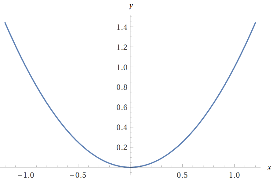
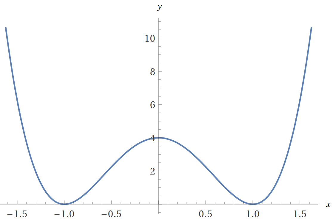
Next, we study the problem of minimizing \(f(x)\) on its domain. It is reasonable to expect that symmetric functions are minimized at the fixed-points of its symmetry. Even functions such as \(f(x) = x^2\) are indeed minimized at the fixed-point \(x=0\), but this is not true for all even functions. For example, \(g(x) = ((1+x)^2+(1-x)^2-4)^2\) is an even function minimized at \(x= \pm 1\), not at \(x=0\).

Thus, we need more structure to guarantee that a symmetric function is minimized at the fixed-points of the symmetry.

Symmetry and convexity

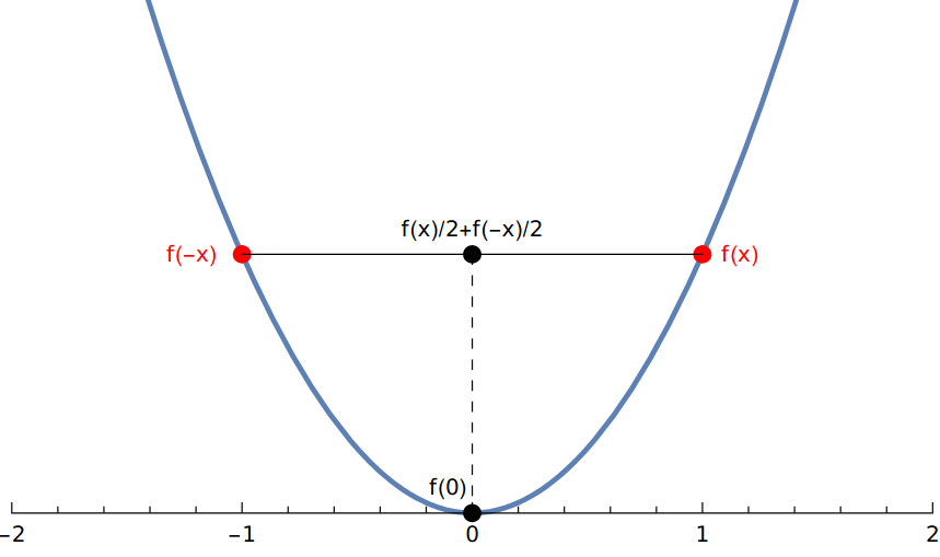
In the example above where \(\symt(x) = -x\), if \(f(x)\) is even and convex, we can show \(f(x)\) is minimized at \(x=0\). The proof is a simple application of the definition of a convex function. For any \(x \in \R\),

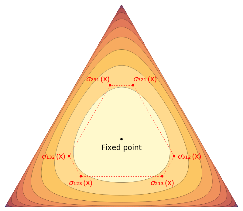
Can we generalize this argument to more complex symmetries and multivariate functions? For our next example, we want to maximize the geometric mean (a concave function) on the simplex \(\Delta_n = \{ x \in \R^n \mid x_i \ge 0,\, \sum_i x_i = 1\}\):

Here \(GM(x)\) has permutation symmetry, where for all \(x \in \Delta_n\) and \(\sigma \in \pi_n\) (the set of all permutations of length \(n\)) we have

Indeed, the only fixed-point in \(\Delta_n\) with respect to permutation symmetry is \(x= \paren{\frac{1}{n},\ldots,\frac{1}{n}}\). By a similar averaging argument using Jensen’s inequality (since \(GM\) is concave), we can show that \(\max_{x \in \Delta_n } GM(x)\) is achieved this fixed-point: For any \(x \in \Delta_n\),

Symmetry reduction using representation theory

The ideas of the previous section can be further generalized using the language of representation theory.

Definition (Group representation) Let \(G\) be a group, \(V\) be a vector space and \(GL(V)\) be the group of non-singular linear transformations over \(V\). A representation of a group \(G\) on \(V\) is a group homomorphism \(\rho: G \rightarrow GL(V)\), such that for all \(g, h \in G\),

For example, one representation of the permutation group \(G=\pi_n\) on the vector space \(V=\R^n\) maps each permutation to an \(n \times n\) permutation matrix.

Definition (Invariant function): A function \(f(x)\) is invariant with respect to a representation \(\rho\) if \(f(\rho(g)x) = f(x)\) for all \(g\in G\) and \(x\) in its domain.

The above definition assumes that \(f\) is unconstrained, but we can easily extend it to constrained optimization problems using indicator functions for the constraint sets.

Definition (Fixed-point subspace): Given representation \(\rho\), the Reynolds operator \(R: V\rightarrow V\) is the linear map:

The fixed-point subspace of \(\rho\) is the image of \(V\) under \(R\):

We can think of \(R_\rho(x)\) as a symmetrizing projection map that sends any point \(x\) to a fixed-point obtained by averaging over all the symmetries of \(G\) applied to \(x\) through representation \(\rho\). Proving that \(R_\rho(V) = \mathcal{F}_\rho\) is left as an exercise for the reader. Generalizing the averaging argument in the earlier examples, we get:

Theorem (Symmetry reduction): If a function \(f(x)\) is convex and invariant with respect to \(\boldsymbol{\rho}\), then it is minimized in the fixed-point subspace \(\mathcal{F}_\rho\).

Symmetry reduction lets us reduce the domain of an optimization problem to a fixed-point subspace. This also reduces the size of the problem, as we shall see in the applications below.

Application: Using symmetries to bound inequalities

One application of symmetry reduction in my research on approximating the permanent of PSD matrices is to find a tight upper bound for the following expectation, where \(x_i \sim N(0, 1)\) are i.i.d. Gaussians and \(\lambda \in \Delta_n\).

This expression comes from analyzing a randomized rounding procedure for a SDP relaxation. We wanted a bound that is tighter than simply applying Jensen’s inequality to get \(f(\lambda) \le 0\). The key is to notice that \(f(\lambda)\) is a concave function on the simplex \(\Delta_n\), which can be proven by standard arguments. After applying symmetry reduction, we get:

where \(\psi\) is the digamma function. This is a tighter bound than simply applying Jensen’s inequality, since \(\psi(\frac{n}{2}) - \log(\frac{n}{2}) < 0\) for all \(n > 0\).

Application: Symmetry reduction in semidefinite programs

A semidefinite program can be written as:

Where \(S_n^+\) is the cone of semidefinite matrices and \(L \subseteq S_n\) is an affine subspace of symmetric \(n \times n\) matrices. In our cases of interest, the action of a group on the space of semidefinite matrices acts on the variables that indexes a quadratic form, thus the fixed-point subspace is defined as:

These fixed-point subspaces for semidefinite matrices have a very specific form: \(F\) will become block diagonal after a change of coordinates. This comes from us being able to write the representation \(\rho\) as a direct sum of irreducible representations. We will not formally prove this and refer readers to Section 4 of Gatermann and Parrilo. An important consequence of this transformation is that the optimization variable matrix \(X\) is replaced with smaller individual blocks, thus reducing the size of the problem.

Example (Cyclic symmetry in SDPs): We consider a SDP with cyclic symmetry, where \(C_i\) are invariant under simultaneous cyclic shifts of the rows and columns.

Such structure can arise in SDP relaxations of graph problems (e.g. max cut, independence number, coloring) on cycle graphs. The group associated with this symmetry is the cyclic group \(C_n\), and \(\mathcal{F}_\rho\) is the space of symmetric matrices that are invariant under cyclic shifts:

These matrices are also known as circulant matrices. In particular, the Fourier basis diagonalizes these matrices, thus we only need to consider the diagonal of \(X\) in this new basis. By doing so we transform the semidefinite constraint into a linear constraint, and reduce the number of variables from \(O(n^2)\) to \(O(n)\).

Generalized reductions to invariant subspaces

Symmetry reductions are not the only type of reductions we can use to reduce the size of an optimization problem. The machinery we developed for symmetry reduction — showing that a problem’s optima lies in an invariant subspace — can be further generalized.

Recall that \(P\) is an orthogonal projection when \(P = P^\top\) and \(P^2 = P\). If a function \(g\) is invariant under an orthogonal projection to a subspace, we can optimize over the image of \(P\) instead (i.e. the subspace that \(P\) projects onto). We obtain the following representer theorem:

Theorem (invariance reduction) Let \(f(w) = g(w) + \frac{1}{2} \norm{w}^2\) be a function on a Hilbert space \(V\). If \(g\) is invariant under an orthogonal projection \(P\), then:

Proof: We show that for all \(w \in V\), \(f(Pw) \le f(w)\), hence we can restrict the domain to \(\im(P) = \{w \in V \mid Pw = w \}\). Since \(g(Pw) = g(w)\), we only need to show that \(\norm{Pw} \le \norm{w}\). Using the Cauchy-Schwarz inequality, we get:

Notice here that \(g\) does not even need to be convex, only invariant under \(P\). Next, we shall see how to use invariance reductions to derive the kernel trick used in many machine learning problems.

Application: Kernel trick as invariant subspace reduction

Consider the ridge regression problem, where we are given \(n\) datapoints \((x_i, y_i)\) and wish to fit a linear model \(y = w^\top x\) with an \(\ell_2\) regularization term weighted by \(\lambda\). This results in the following convex optimization problem:

When \(d \gg n\), we are in a regime where the dimension \(d\) of \(x_i\) and \(w\) is much larger (possibly infinite) than the number of datapoints \(n\). However, we can drastically reduce the size of the problem with the following observation:

Proposition (Invariance under projection): Let \(P\) be the orthogonal projection onto the subspace spanned by \(x_1, \ldots, x_n\) and \(g(w) = \sum_{i=1}^n (\dotp{x_i, w} - y_i)^2\). For any \(w\) we have:

Thus by invariance reduction, we can instead minimize f(w) on the span of the data \(x_1, \ldots, x_n\). This is a (much smaller) subspace of dimension \(n\). In fact, we can parameterize this subspace with a linear combination of the data:

Making this substitution back into the optimization problem, we get:

Where \(K = X^\top X \in \R^{n \times n}\) is the kernel matrix with size determined by the number of \(x_i\), not the dimension of \(x_i\). The solution has a closed form, \(c = (K + \lambda I)^{-1} y\). Thus, we can see that the kernel trick is an application of invariance reduction using orthogonal projections onto the span of data. The procedure of restricting the domain of an optimization problem to the span of data then replacing \(\dotp{x_i, x_j}\) with \(K_{ij}\) is called kernelization.

I think this is a more natural way of deriving kernel ridge regression than the usual method of first writing down the normal equation to get \(X^\top w = X^\top (X X^\top + \lambda I)^{-1} X y\), then using the identity \((X X^\top + \lambda I)^{-1} X = X (X^\top X + \lambda I)^{-1}\). These two different methods and their equivalence are summarized in the diagram below:

Next we look at classification with Support Vector Machines (SVMs), which finds a separating hyperplane given linearly separable data \(x_i\) from two classes \(y_i \in \{\pm 1\}\) by solving the following optimization problem:

Since the constraints are invariant under orthogonal projection to the span of the data \(x_i\), we can apply the same invariance reduction as before (substituting \(w = Xc\)) to reduce its dimension.

Typically, deriving kernel SVM requires taking the dual of the above optimization problem, so that \(\dotp{x_i, x_j}\) appears in the objective. This suggests that the dual formulation is essential for the kernel trick to work. In the diagram below, we see that this is not the case: Kernelization (invariance reduction) can be applied to both the primal and dual forms of the problem, and the resulting reduced-size problems are dual to each other.

Where \(X = [ x_1 \cdots x_n]\), \(K_{ij} = \dotp{x_i, x_j}\), \(K_i\) is the \(i\)-th column of \(K\), and \(\circ\) denotes the element-wise Hadamard product.

References and other resources

This article is partly based on my scribe notes of Pablo Parrilo’s lecture for the class Proofs, beliefs and algorithms through the lens of Sum of Squares in Fall 2016.

Do symmetric problems have symmetric solutions? Waterhouse (1983)

Symmetry groups, semidefinite programs, and sums of squares. Gatermann & Parrilo (2004)

Reduction methods in semidefinite and conic optimization. Permenter (2017)

A generalized representer theorem. Schölkopf, Herbrich, & Smola (2001)

A unifying view of representer theorems. Argyriou & Dinuzzo (2014)