NP Completeness

Let’s look at an algorithmic problem. We have a graph, and we want to color all the vertices with 2 colors such that each edge connects 2 vertices of the same color. This problem is called \(\text{2-coloring}\). An example of a 2-colorable graph is shown below.

Can we devise an efficient algorithm that determines whether a graph is 2-colorable, and outputs a 2-coloring if it is? It turns out that we can do this easily by first assigning an arbitrary color to any node, then continue assigning colors to adjacent nodes while making sure no edge joins 2 vertices of the same color, until either all the nodes have a color (successful), or a contradiction is reached (failure). This algorithm runs in time proportional to the size of the graph. Notice that the only time we need to make a choice in coloring is for the first node. After this, the colors of the remaining nodes are fixed, constrained by the problem.

Now let’s look at the above graph. This graph cannot be colored with 2 colors but can be colored with 3. If we have any graph, is there an efficient algorithm to solve \(\text{3-coloring}\)? If we try to modify the algorithm for \(\text{2-coloring}\), we immediately see a problem. With the additional color, after choosing a color for the first vertex, we are faced with a choice of 2 colors for any adjacent vertex. It’s this extra choice that makes this problem hard, eluding efficient solution for decades.

Many problems, such as \(\text{3-coloring}\), do not have an efficient solution even after many smart people pondered over them for years. These problems became known as hard problems. But how do we exactly quantify hardness? This is going to be the objective of this post.

First, we would look at search problems, problems whose solutions can be verified in polynomial time, which is a more precise way of saying “efficiently”. For example, although \(\text{3-coloring}\) is difficult to solve, we can efficiently verify if a given coloring is a 3-coloring. First we check that there are 3 colors used, then we check that each edge connects 2 vertices of different colors, taking time proportional to the size of the graph. Using this verifier, we have another way to solve this problem: enumerate all the possible 3-colorings, then use the verifier to check if any is valid. However for a graph with \(n\) vertices, there are \(3^n\) possible colorings, so this isn’t an efficient solution.

We call the set of search problems, problems that can be efficiently verified, NP. We also call the set of problems that can be solved in polynomial time P. It is a million-dollar open problem to tell if these two sets are equal.

We do not know if all search problems can be efficiently solved, but we do have a way of comparing the relative difficulty of problems. This technique is called reduction. Suppose we have two problems, \(A\) and \(B\), and we have a solver for \(A\). If we can somehow modify all instances of \(B\) such that they can be solved with \(A\)’s solver, we say that \(B\) can be reduced to \(A\). We use an arrow to denote this reduction: \(B \rightarrow A\). Also, this means that \(A\) is at least as hard as \(B\), since \(A\)’s solver can be used to solve \(B\).

For a concrete example, let’s try to find a reduction from \(\text{3-coloring}\) to \(\text{4-coloring}\). Suppose we have a solver for \(\text{4-coloring}\), and we want to modify a 3-coloring problem such that the solver will give us a solution if the graph is 3-colorable, and tells us if it is not. Specifically, we need to handle the case where the graph is 4-colorable but not 3-colorable. The solver has an additional color to work with, but we don’t want to use that color in the original graph. Thus we modify it by adding an additional vertex and connecting it to all other vertices in the original graph. It is then easy to verify that the \(\text{4-coloring}\) solver will give a solution if and only if the original graph is 3-colorable. This can be generalized by induction to \(n\text{-coloring}\).

Now we have a method to compare the difficulty of problems, we can say that two problems have the same difficulty if they can be reduced efficiently to one another. It turns out that some problems are the hardest problems in NP. This means that every single problem in NP reduces to them. These problems are called NP-complete. How do we prove that a problem is NP-complete?

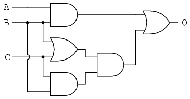
Let’s start by looking at two other problems, \(\text{3-SAT}\) and \(\text{Circuit-SAT}\). In \(\text{3-SAT}\), we are given a series of clauses joined by and, where each clause is up to 3 variables or their negation joined by or. For example, \((x \vee y \vee \bar{z}) \wedge (\bar{x} \vee y)\). We need to find an assignment to each variable, either \(T\) or \(F\), such that the entire expression evaluates to \(T\), or say that it is impossible to do so. In \(\text{Circuit-SAT}\), we are given a network of Boolean circuits with many inputs and one output, and our task is to find a set of inputs such that the output of the circuit is \(T\), or say that it’s impossible to do so. An example of a Boolean circuit is shown below.

With these problems defined, we can follow this path of reductions to prove that \(n\text{-coloring}\) is NP-complete.

We have already done the last reduction, and would not be doing \(\text{3-SAT} \rightarrow \text{3-coloring}\). Interested readers can read these lecture notes for details. \(\text{Circuit-SAT} \rightarrow \text{3-SAT}\) can be done by converting each gate to logic clauses. For example, an and-gate with inputs \(x_1\), \(x_2\) and output \(y\) can be converted into \((x_1 \wedge x_2) \iff y\) and simplified into the desired form with Boolean algebra.

The most interesting reduction in this stack is \(\text{All of NP} \rightarrow \text{Circuit-SAT}\). Recall that to prove this reduction, suppose we have a \(\text{Circuit-SAT}\) solver, we need to find a way to use this solver to solve any problem in NP. Since a problem in NP is a search problem, it must have an efficient verifier. This verifier is a program that takes a solution and outputs “True” if the solution is valid, or “False” if it isn’t. This program can be implemented on a computer, which itself is a network of Boolean circuits! Thus there is a way to convert this program into a circuit to feed into the \(\text{Circuit-SAT}\) solver, and we have shown that \(\text{Circuit-SAT}\) and all the other problems in this chain is at least as hard as any other problem in NP, thus are NP-complete.

In this post, I’ve talked about the notion of NP-completeness, and using reduction as a tool to prove NP-completeness. People have shown that many more problems are NP-complete, and this is just the tip of the iceberg which is complexity theory. In a future post, I’ll talk about methods to cope with NP-complete problems and SAT solvers.